Kernel Density Plot

Kernel Density Plot is a graphical tool that visually represents data distribution. By smoothing data points, it creates a continuous probability density function, helping users better understand the data distribution. SPSSAU supports the following functions:

Batch add 'titles' for plotting.

Add categorical variables (e.g., gender) to generate kernel density plots for different categories.

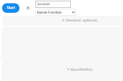
Users can choose different kernel functions.

The system automatically sets the bandwidth , but users can also customize one.

Data Format

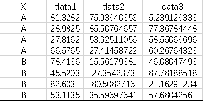
The dataset includes one Category and the analysis data. Category can be omitted during analysis if not needed.

Calculation Steps

1.Data Preparation

Collect a sample dataset: x₁, x₂, ..., x_n.

2.Select a Kernel Function

Choose an appropriate kernel function that satisfies {\int }_{-\mathrm{\infty }}^{\mathrm{\infty }}K(x)dx=\mathit{1}. SPSSAU provides the following kernel functions: Uniform, Triangular, Epanechnikov, Quartic, Gaussian, and Cosine. Gaussian is the default function.

Kernel Function	Formula
Uniform	$$K(x)=\{\begin{array}{c}\frac{1}{2},x\in [-1,1]\\ 0,\text{ Others }\end{array}$$
Triangular	$$K(x)=\{\begin{array}{c}1-\left|x\right|,x\in [-1,1]\\ 0,\text{ Others }\end{array}$$
Epanechnikov	$$K(x)=\{\begin{array}{c}\frac{3}{4}(1-x^2),x\in [-1,1]\\ 0,\text{ Others }\end{array}$$
Quartic	$$K(x)=\{\begin{array}{c}\frac{15}{16}{(1-x^2)}^2,x\in [-1,1]\\ 0,\text{ Others }\end{array}$$
Gaussian [default]	$$K(x)=\frac{1}{\sqrt{2\pi }}{e}^{\frac{x^2}{2}},x\in R.$$
Cosine	$$K(x)=\{\begin{array}{c}\frac{\pi }{4}\cos \frac{\pi }{2}x,x\in [-1,1]\\ 0,\text{ Others }\end{array}$$

3.Choose Bandwidth

Select an appropriate bandwidth (h > 0) to control the smoothness of the kernel function. The smaller the bandwidth, the less smooth the estimation. SPSSAU uses 'Silverman's Rule of Thumb' by default to calculate h:

$$h=(\frac{3\times n}{4}{)}^{-\frac{1}{5}}\times min(s,\frac{IQR}{1.35}).$$

• s represents the sample standard deviation.
• IQR represents the interquartile range.
• n represents the sample size.
• min selects the smaller value between the two.

4.Calculate Kernel Density Estimation

For any given x,\hat{f}(x) is defined as:

$$\hat{f}(x)=\frac{\mathit{1}}{\mathit{n}\mathit{h}}\sum _{\mathit{i}\mathit{=}\mathit{1}}^{\mathit{n}}\mathit{K}\mathit{(}\frac{\mathit{x}\mathit{-}{\mathit{x}}_{\mathit{i}}}{\mathit{h}}\mathit{)}$$

5.Plot the Kernel Density Plot

Plot \hat{f}(x) to generate the kernel density plot.